1.Utilizing Real-World Examples in scPagwas for Comprehensive Testing
To showcase the visualization effects accurately, we have opted to use real-world examples from the referenced article instead of the software’s provided demo dataset. In this scenario, we will be utilizing the BMMC scRNA-seq data in conjunction with the GWAS data for monocyte count. It is important to note that due to the large size of the data, the computation time for this analysis may take several minutes. Hence, we recommend directly downloading the result data for convenient examination and exploration. The processed monocytecount gwas data can be download from:
-
Onedrive: https://1drv.ms/t/s!As-aKqXDnDUHi6sx7Hqblj2Sgl7P8w?e=pwSq1Q
-
BaiduCloud: https://pan.baidu.com/s/1Ce1vvd-u_ckllWOeDtAXkw?pwd=1234
BMMC example scRNA-seq data can be obtained from:
-
Ondrive: https://1drv.ms/u/s!As-aKqXDnDUHjfcMjN4VGtAw1Utm0w?e=bOOBJl
-
BaiduCloud: https://pan.baidu.com/s/1iarcexEBOflne86BblaOhg?pwd=1234
We can download the result files from:
-
Ondrive: https://1drv.ms/u/s!As-aKqXDnDUHjLNvq64d2GAK_pIGVA?e=bZSawC
-
BaiduCloud: https://pan.baidu.com/s/1rB5iRvXTyHIZfQUFr7eGDw?pwd=1234
Code: 1234
If you want to run the demo data, please go to Conventional Usage Instructions for scPagwas with Demo Example Data
2. Computing the singlecell and celltype result for Monocytecount trait
If we running scPagwas in multi-core in server environment, there may cause an error: Error: Two levels of parallelism are used. See ?assert_cores\` add this code before call in R environment:
export OPENBLAS_NUM_THREADS=1
There is no need to run this code in window system.
In this example, we run the scPagwas for usual step, both running singlecell and celltype process.
library(scPagwas)
Pagwas<-scPagwas_main(Pagwas =NULL,
                     gwas_data="monocytecount_prune_gwas_data.txt",
                     Single_data ="Seu_Hema_data.rds",
                     output.prefix="mono",
                     output.dirs="monocytecount_bmmc",
                     Pathway_list=Genes_by_pathway_kegg,
                     n.cores=2,
                     assay="RNA",
                     singlecell=T,
                     iters_singlecell = 100,
                     celltype=T,
                     block_annotation = block_annotation,
                     chrom_ld = chrom_ld)
save(Pagwas,file="./BMMC_scPagwas.RData")
Sometimes, we need to remove the objects in cache folder:
if(length(SOAR::Objects())>0){
 SOAR::Remove(SOAR::Objects())
}
3. Result interpretation
Data Results and Output in scPagwas:
- By default (seurat_return = TRUE), scPagwas returns the data results in Seurat format, which ensures consistency with the input single-cell data format. The scPagwas results in Seurat format include two additional assays, five new columns in the meta.data, and five new columns in the misc data.
- In the output folder, there will be five result files along with an empty folder named “scPagwas_cache”. Generally, the “scPagwas_cache” folder is unnecessary and can be deleted without affecting the results.
3.1 Pagwas
> print(Pagwas)
An object of class Seurat
16478 features across 35582 samples within 3 assays
Active assay: RNA (15860 features, 5000 variable features)
 2 other assays present: scPagwasPaHeritability, scPagwasPaPca
 3 dimensional reductions calculated: pca, tsne, umap

> names(Pagwas@misc)
[1] "Pathway_list"                  "pca_cell_df"                   "lm_results"
[4] "bootstrap_results"             "scPathways_rankPvalue"         "GeneticExpressionIndex"
[7] "Merged_celltype_pvalue"
-
In this Seruat result, two new assays were added:
-
scPagwasPaPca: An assay for S4 type of data; the svd score result for pathways in each cells;
-
scPagwasPaHeritability: An assay for S4 type of data; the gPas score matrix for pathways in each cells;
-
These two files are intermediate files generated by scPagwas.
-
In meta.data, four columns were added:
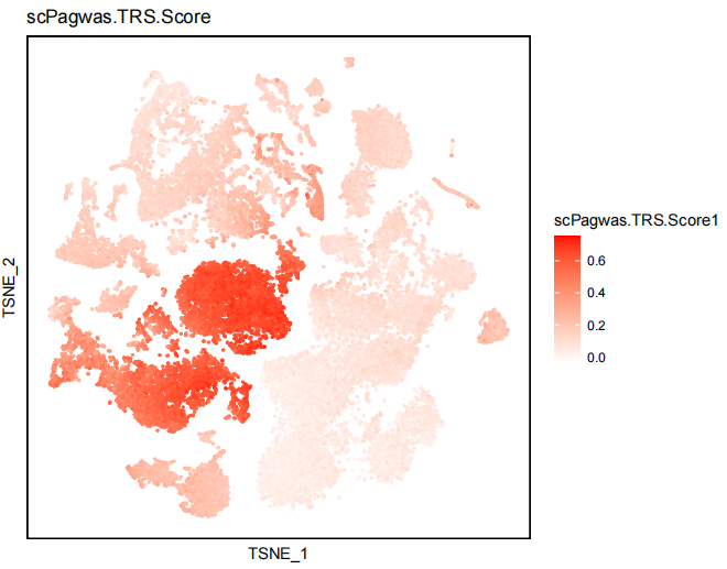
- scPagwas.TRS.Score1: inheritance related score, enrichment socre for genetics top genes;
- scPagwas.downTRS.Score: Trait relevant score based on anti-genetic relevant genes
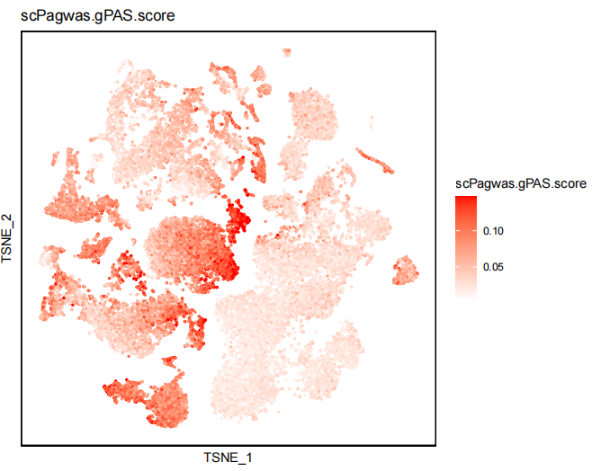
- scPagwas.gPAS.score: Inheritance pathway regression effects score for each cells;
- Random_Correct_BG_p: Cell pValue for TRS score of each cells;
- Random_Correct_BG_adjp: fdr for each cells, adjust p value.
- Random_Correct_BG_z:z score for eahc cells.
-
A new element names misc is added in scPagwas’s result,
Pagwas@miscis a list including:-
Pathway_list: filtered pathway gene list;
-
pca_cell_df: a pahtway and celltype data frame for pathway svd(1’st pca) result for each celltype;
-
lm_results: the regression result for each celltype;
-
PCC: pearson correlation coefficients,heritability correlation value for each gene;
-
bootstrap_results: The bootstrap data frame results for celltypes including bootstrap pvalue and confidence interval.
-
Merged_celltype_pvalue: The resulting Merged_celltype_pvalue represents p-values at the cell type level, which differ from the bootstrap_results. The bootstrap_results are based on merging cell-level expression data into cell type-level expression data and performing calculations. In contrast, the Merged_celltype_pvalue is derived from the Random_Correct_BG_p results, combining the p-values of all cells within a specific cell type into a single p-value result for that cell type.
Note: Although both the bootstrap and merged strategies yield cell type-level results, they may not be identical. This is because the bootstrap approach calculates p-values based on pseudo-bulk data, which can differ from the results obtained from single-cell calculations. In contrast, the merged strategy directly integrates the results from single-cell calculations, resulting in greater consistency with single-cell results. The primary focus in scPagwas paper is on the bootstrap_results; however, during the later stages of development, we discovered that discrepancies between cell type-level and single-cell-level calculation strategies posed some challenges in downstream analyses. Hence, in the new version development, we directly utilize the integration of single-cell results to obtain cell type-level p-values. Additionally, the major advantage of the bootstrap_results is its speed, as the calculation of Random_Correct_BG_p for single cells requires at least 100 iterations, making it computationally demanding. To avoid calculating Random_Correct_BG_p, setting the parameter iters_singlecell=0 is a good option.
3.2 Pagwas : output files result
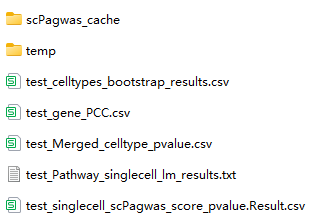

In monocytecount_bmmc folder, There is several result files :
-
*_cellytpes_bootstrap_results.csv : The result of cellytpes for bootstrap p results;
-
*_gene_PCC.csv : The result of gene expression correlation with gPAS score.
- *_Pathway_singlecell_lm_results.txt : The regression result for all pahtway and single cell matrix;
- *_singlecell_scPagwas_score_pvalue.Result.csv : The data frame result for each cell inlcuding scPagwas.TRS.Score, scPagwas.downTRS.Score, scPagwas.gPAS.score, pValueHighScale, qValueHighScale;
- *_Merged_celltype_pvalue.csv : The merged singlecell pvalue to celltype pvalue.
- scPagwas_cache is a temporary folder to save the SOAR data, you can remove it when finish the scPagwas.
-
-
4. Result Visualization
4.1 Visualize the scPagwas Score of single cell data in UMAP or TSNE plot.
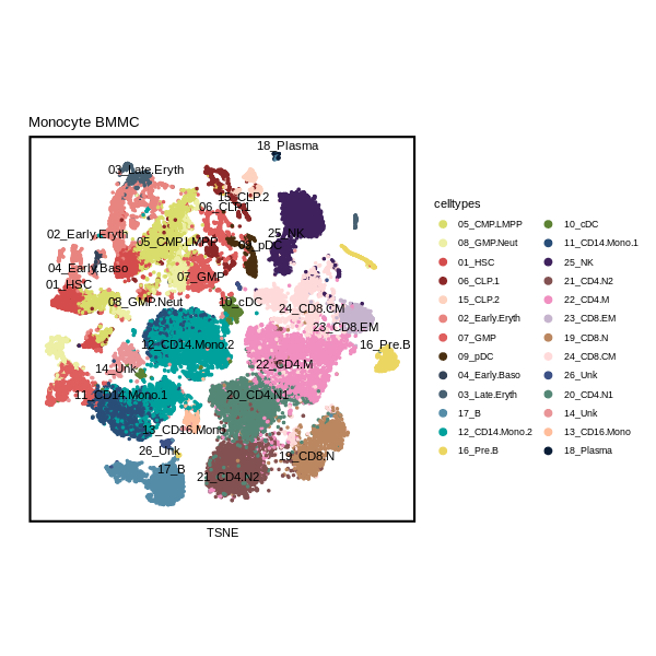
1) DimPlot of singlecell data.
 require("RColorBrewer")
 require("Seurat")
 require("SeuratObject")
 require("ggsci")
 require("dplyr")
 require("ggplot2")
 require("ggpubr")
 #check the objects
color26 <- c("#D9DD6B","#ECEFA4","#D54C4C","#8D2828","#FDD2BF","#E98580","#DF5E5E","#492F10","#334257","#476072","#548CA8","#00A19D","#ECD662","#5D8233","#284E78","#3E215D","#835151","#F08FC0","#C6B4CE","#BB8760","#FFDADA","#3C5186","#558776","#E99497","#FFBD9B","#0A1D37")

Seurat::DimPlot(Pagwas,pt.size=1,reduction="tsne",label = T, repel=TRUE)+
 scale_colour_manual(name = "celltypes", values = color26)+
 umap_theme()+ggtitle("Monocyte BMMC")+labs(x="TSNE",y="")+theme(aspect.ratio=1)
 scPagwas.TRS.Score1 and positive(p<0.05) cells showing in dimplot.
 scPagwas_Visualization(Single_data=Pagwas,
                        p_thre = 0.05,
                        FigureType = "tsne",
                        width = 7,
                        height = 7,
                        lowColor = "white",
                        highColor = "red",
                        output.dirs="figure",
                        size = 0.5,
                        do_plot = T)
2) scPagwas.gPAS.score dimplot.
3) scPagwas.TRS.Score dimplot.
4) Random_Correct_BG_adjp dimplot.
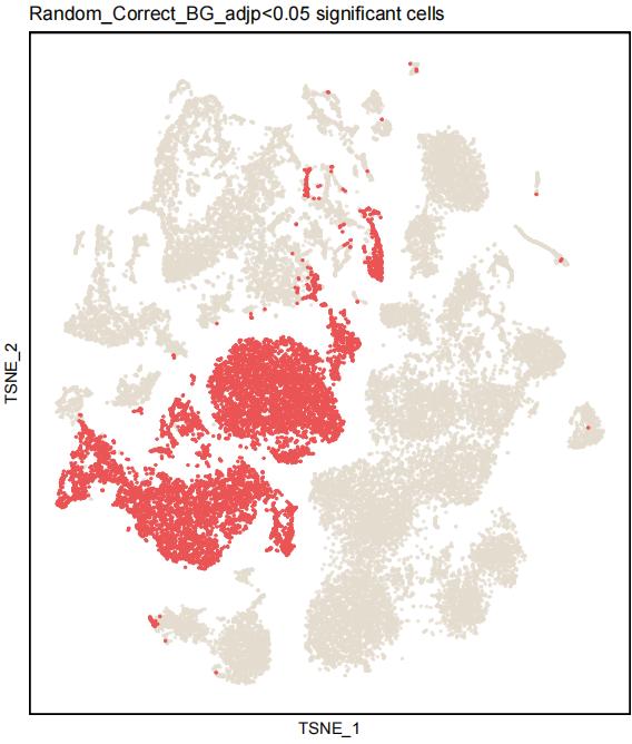
Positive cells(Random_Correct_BG_adjp<0.05): red dot; Negative cells: other dot.
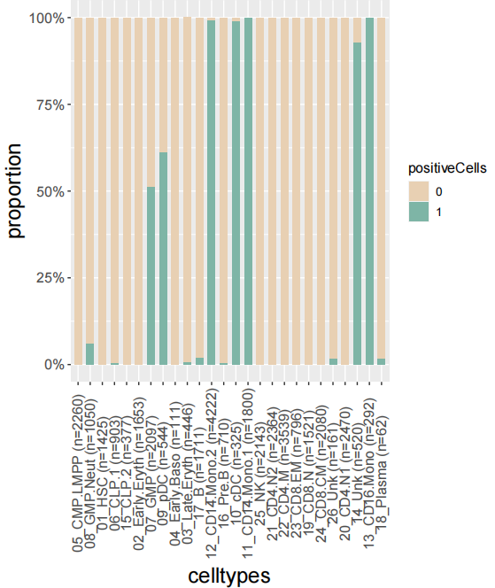
4.2 Plot the barplot of the proportion of positive Cell.
Plot the barplot of the proportion of positive Cells in celltypes:
plot_bar_positie_nagtive(seurat_obj=Pagwas,
                         var_ident="celltypes",#you should change this to you specific columns
                         var_group="positiveCells",
                         vec_group_colors=c("#E8D0B3","#7EB5A6"),
                         do_plot = T)
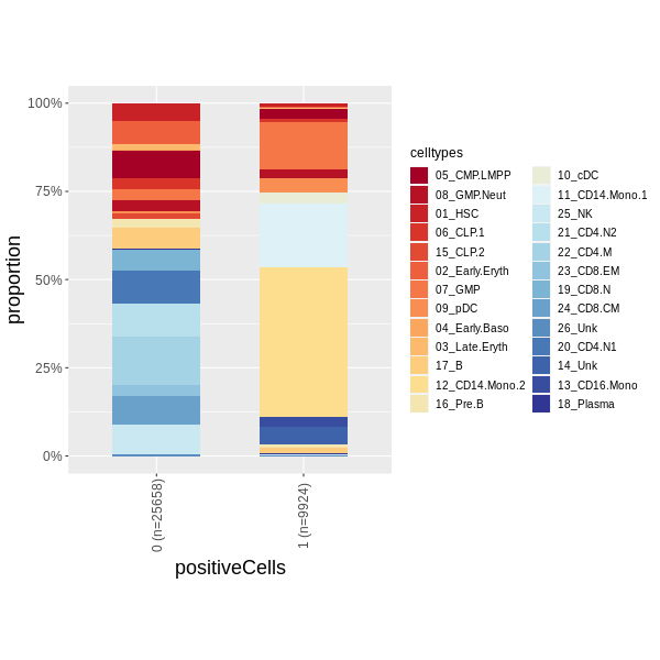
 Plot the barplot of the proportion of celltypes in positive and negative Cells:
pdf("D:/OneDrive/RPakage/scPagwas/vignettes/figures/plot_bar_positie_nagtive.pdf")
plot_bar_positie_nagtive(seurat_obj=Pagwas,
                              var_ident="positiveCells",
                              var_group="celltypes", #you should change this to you specific columns
                              p_thre = 0.01,
                              vec_group_colors=NULL,
                              f_color=colorRampPalette(brewer.pal(n=10, name="RdYlBu")),
                              do_plot = T)
dev.off()
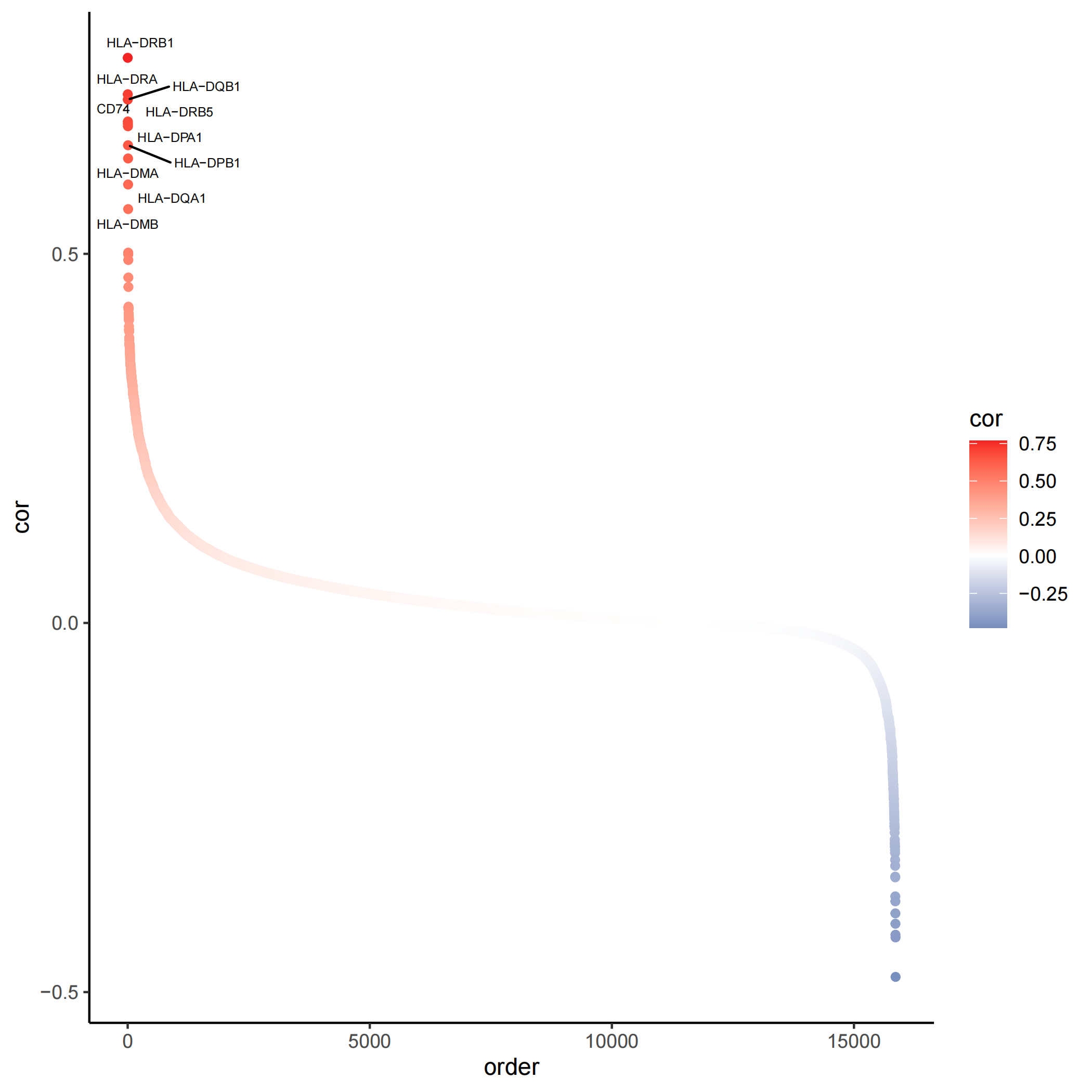
4.3 Plot the heritability correlated genes
heritability_cor_scatterplot(gene_heri_cor=Pagwas@misc$PCC,
                             topn_genes_label=10,
                             color_low="#035397",
                             color_high ="#F32424",
                             color_mid = "white",
                             text_size=2,
                             do_plot=T,
                             max.overlaps =20,
                             width = 7,
                             height = 7)
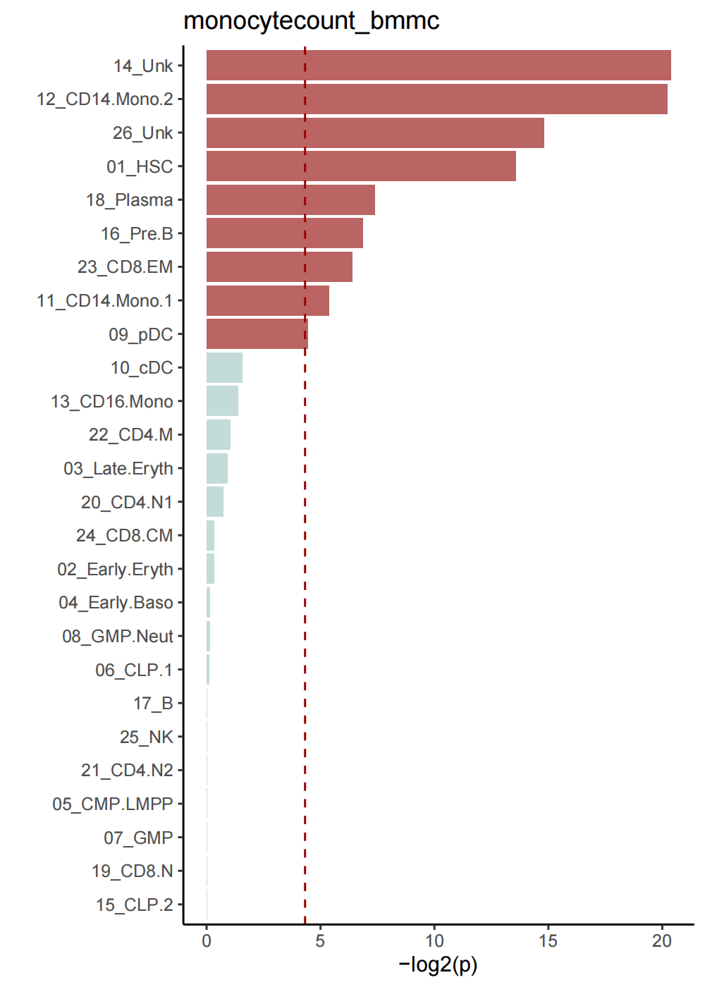
4.4 celltypes bootstrap_results reuslt
Barplot for celltypes
Bootstrap_P_Barplot(p_results=Pagwas@misc$bootstrap_results$bp_value[-1],
                    p_names=rownames(Pagwas@misc$bootstrap_results)[-1],
                    figurenames = "Bootstrap_P_Barplot.pdf",
                    width = 5,
                    height = 7,
                    do_plot=T,
                    title = "monocytecount_bmmc")
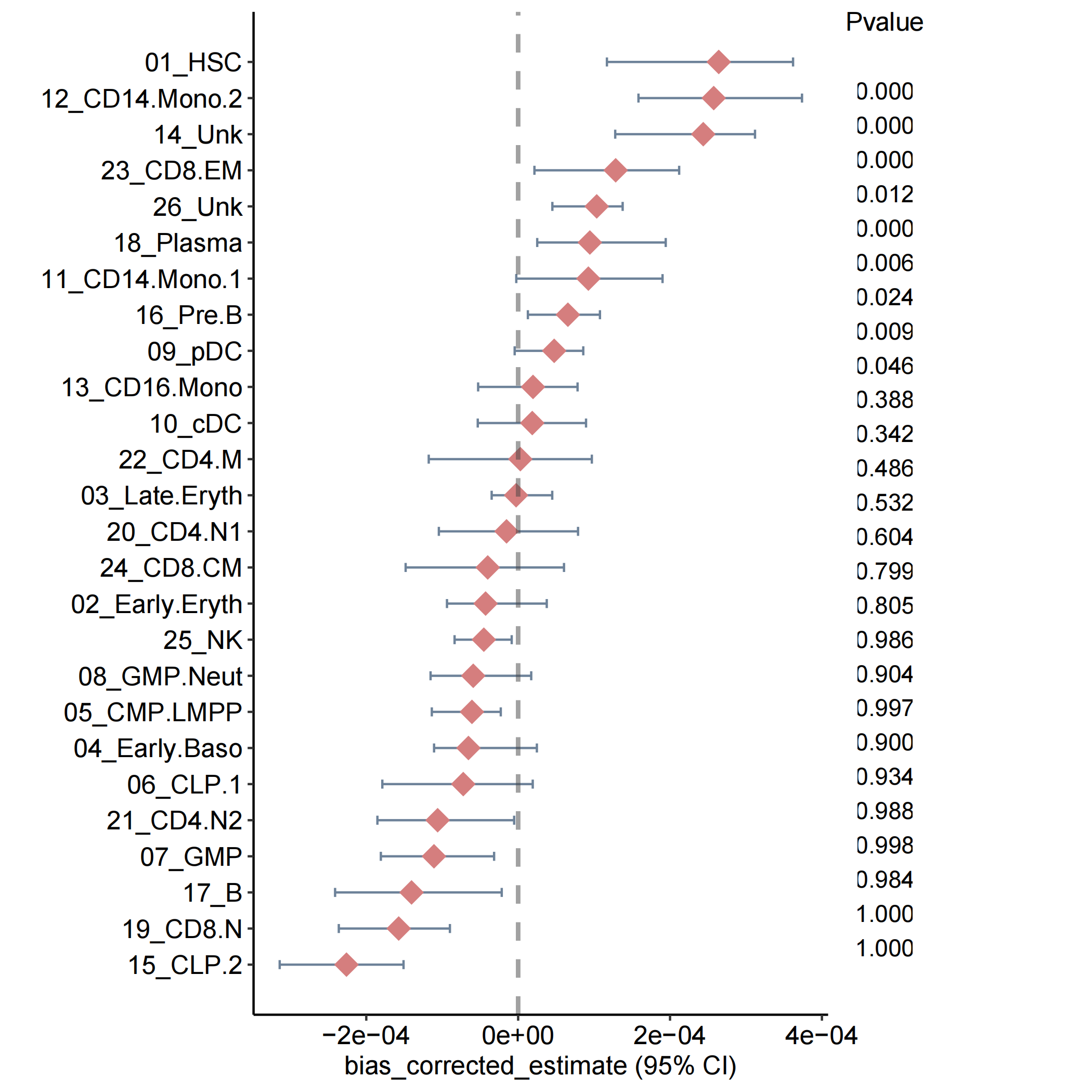
Forest plot for estimate value.
Bootstrap_estimate_Plot(bootstrap_results=Pagwas@misc$bootstrap_results,
                        figurenames = "estimateplot.pdf",
                        width = 9,
                        height = 7,
                        do_plot=T)
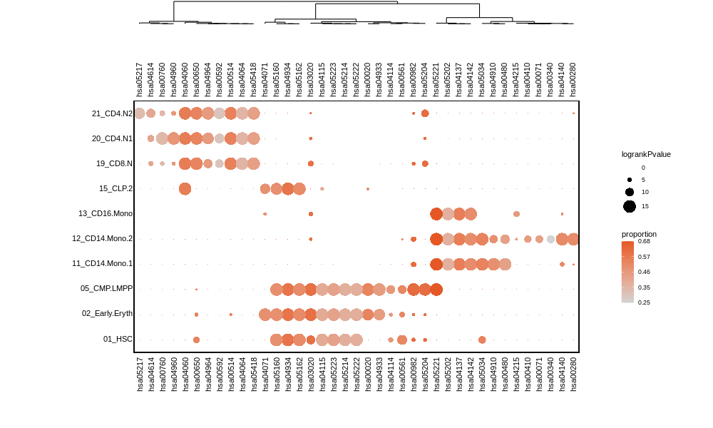
4.5 Visualize the heritability correlated Pathways
Plot the specific genetics pathway for each celltypes
library(tidyverse)
library("rhdf5")
library(ggplot2)
library(grDevices)
library(stats)
library(FactoMineR)
library(scales)
library(reshape2)
library(ggdendro)
library(grImport2)
library(gridExtra)
library(grid)
library(sisal)

source(system.file("extdata", "plot_scpathway_contri_dot.R", package = "scPagwas"))
plot_scpathway_dot(Pagwas=Pagwas,
                   celltypes=c("01_HSC","02_Early.Eryth","05_CMP.LMPP","11_CD14.Mono.1","12_CD14.Mono.2","13_CD16.Mono","15_CLP.2","19_CD8.N","20_CD4.N1","21_CD4.N2"),
                   topn_path_celltype=5,
                   filter_p=0.05,
                   max_logp=15,
                   display_max_sizes=F,
                   size_var ="logrankPvalue" ,
                   col_var="proportion",
                   shape.scale = 8,
                   cols.use=c("lightgrey", "#E45826"),
                   dend_x_var = "logrankPvalue",
                   dist_method="euclidean",
                   hclust_method="ward.D",
                   do_plot = T,
                   width = 7,
                   height = 7)
sessionInfo
R version 4.2.2 (2022-10-31 ucrt)
Platform: x86_64-w64-mingw32/x64 (64-bit)
Running under: Windows 10 x64 (build 22621)

Matrix products: default

locale:
[1] LC_COLLATE=Chinese (Simplified)_China.utf8  LC_CTYPE=Chinese (Simplified)_China.utf8
[3] LC_MONETARY=Chinese (Simplified)_China.utf8 LC_NUMERIC=C
[5] LC_TIME=Chinese (Simplified)_China.utf8

attached base packages:
[1] stats     graphics  grDevices datasets  utils     methods   base

loaded via a namespace (and not attached):
 [1] Rcpp_1.0.9          compiler_4.2.2      RColorBrewer_1.1-3  progressr_0.11.0
 [5] tools_4.2.2         digest_0.6.30       evaluate_0.18       Rtsne_0.16
 [9] lattice_0.20-45     rlang_1.0.6         Matrix_1.5-3        cli_3.3.0
[13] rstudioapi_0.14     yaml_2.3.6          parallel_4.2.2      xfun_0.34
[17] fastmap_1.1.0       knitr_1.40          SOAR_0.99-11        bigreadr_0.2.4
[21] bigassertr_0.1.5    globals_0.16.1      grid_4.2.2          data.table_1.14.4
[25] listenv_0.8.0       future.apply_1.10.0 RcppAnnoy_0.0.20    parallelly_1.32.1
[29] RANN_2.6.1          rmarkdown_2.18      ROCR_1.0-11         codetools_0.2-18
[33] htmltools_0.5.3     MASS_7.3-58.1       future_1.29.0       renv_0.16.0
[37] KernSmooth_2.23-20